
Editor’s note: Full disclosure — the author is a developer and software architect at ArangoDB GmbH, which leads the development of the open source multi-model database ArangoDB.
In recent years, the idea of “polyglot persistence” has emerged and become popular — for example, see Martin Fowler’s excellent blog post. Fowler’s basic idea can be interpreted that it is beneficial to use a variety of appropriate data models for different parts of the persistence layer of larger software architectures. According to this, one would, for example, use a relational database to persist structured, tabular data; a document store for unstructured, object-like data; a key/value store for a hash table; and a graph database for highly linked referential data. Traditionally, this means that one has to use multiple databases in the same project, which leads to some operational friction (more complicated deployment, more frequent upgrades) as well as data consistency and duplication issues.
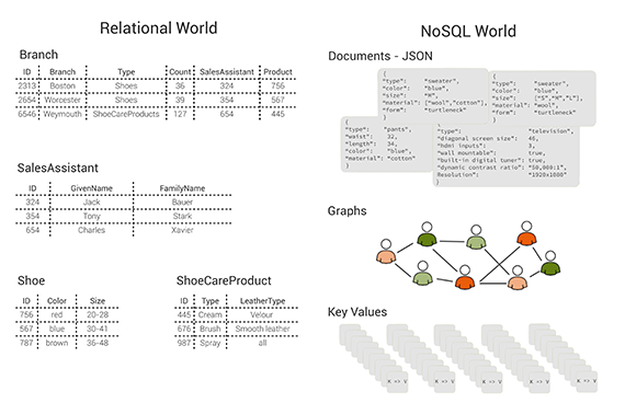
Figure 1: tables, documents, graphs and key/value pairs: different data models. Image courtesy of Max Neunhöffer.
This is the calamity that a multi-model database addresses. You can solve this problem by using a multi-model database that consists of a document store (JSON documents), a key/value store, and a graph database, all in one database engine and with a unifying query language and API that cover all three data models and even allow for mixing them in a single query. Without getting into too much technical detail, these three data models are specially chosen because an architecture like this can successfully compete with more specialised solutions on their own turf, both with respect to query performance and memory usage. The column-oriented data model has, for example, been left out intentionally. Nevertheless, this combination allows you — to a certain extent — to follow the polyglot persistence approach without the need for multiple data stores.
At first glance, the concept of a multi-model database might be a bit hard to swallow, so let me explain this idea briefly. Documents in a document collection usually have a unique primary key that encodes document identity, which makes a document store naturally into a key/value store, in which the keys are strings and the values are JSON documents. In the absence of secondary indexes, the fact that the values are JSON does not really impose a performance penalty and offers a good amount of flexibility. The graph data model can be implemented by storing a JSON document for each vertex and a JSON document for each edge. The edges are kept in special edge collections that ensure that every edge has “from” and “to” attributes that reference the starting and ending vertices of the edge respectively. Having unified the data for the three data models in this way, it only remains to devise and implement a common query language that allows users to express document queries, key/value lookups, “graphy queries,” and arbitrary mixtures of these. By “graphy queries,” I mean queries that involve the particular connectivity features coming from the edges, for example “ShortestPath,” “GraphTraversal,” and “Neighbors.”
Aircraft fleet maintenance: A case study
One area where the flexibility of a multi-model database is extremely well suited is the management of large amounts of hierarchical data, such as in an aircraft fleet. Aircraft fleets consists of several aircraft, and a typical aircraft consists of several million parts, which form subcomponents, larger and smaller components, such that we get a whole hierarchy of “items.” To organise the maintenance of such a fleet, one has to store a multitude of data at different levels of this hierarchy. There are names of parts or components, serial numbers, manufacturer information, maintenance intervals, maintenance dates, information about subcontractors, links to manuals and documentation, contact persons, warranty and service contract information, to name but a few. Every single piece of data is usually attached to a specific item in the above hierarchy.
This data is tracked in order to provide information and answer questions. Questions can include but are not limited to the following examples:
- What are all the parts in a given component?
- Given a (broken) part, what is the smallest component of the aircraft that contains the part and for which there is a maintenance procedure?
- Which parts of this aircraft need maintenance next week?
A data model for an aircraft fleet
So, how do we model the data about our aircraft fleet if we have a multi-model database at our disposal?
There are probably several possibilities, but one good option here is the following (because it allows us to execute all required queries quickly): there is a JSON document for each item in our hierarchy. Due to the flexibility and recursive nature of JSON, we can store nearly arbitrary information about each item, and since the document store is schemaless, it is no problem that the data about an aircraft is completely different from the data about an engine or a small screw. Furthermore, we store containment as a graph structure. That is, the fleet vertex has an edge to every single aircraft vertex, an aircraft vertex has an edge to every top-level component it consists of, component vertices have edges to the subcomponents they are made of, and so on, until a small component has edges to every single individual part it contains. The graph that is formed in this way is in fact a directed tree:
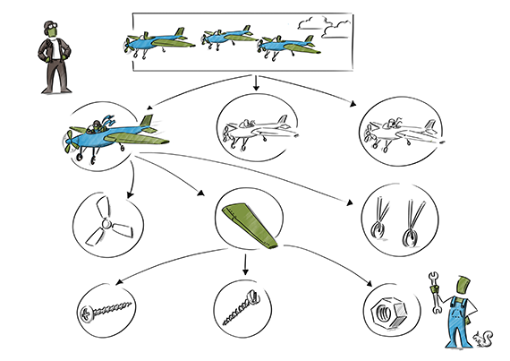
Figure 2: A tree of items. Image courtesy of Max Neunhöffer.
We can either put all items in a single (vertex) collection or sort them into different ones — for example, grouping aircraft, components, and individual parts respectively. For the graph, this does not matter, but when it comes to defining secondary indexes, multiple collections are probably better. We can ask the database for exactly those secondary indexes we need, such that the particular queries for our application are efficient.
Queries for aircraft fleet maintenance
We now come back to the typical questions we might ask of the data, and discuss which kinds of queries they might require. We will also look at concrete code examples for these queries using the ArangoDB Query Language (AQL).
- What are all the parts in a given component?
This involves starting at a particular vertex in the graph and finding all vertices “below” — that is, all vertices that can be reached by following edges in the forward directions. This is a graph traversal, which is a typical graphy query.
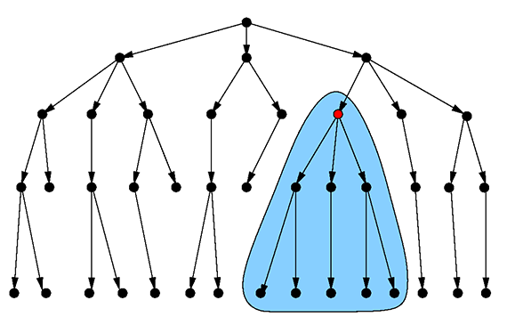
Figure 3: Finding all parts in a component. Image courtesy of Max Neunhöffer.
Here is an example of this type of query, which finds all vertices that can be reached from “components/Engine765” by doing a graph traversal:
RETURN GRAPH_TRAVERSAL("FleetGraph",
                       "components/Engine765",
                       "outbound")
In ArangoDB, one can define graphs by giving them a name and by specifying which document collections contain the vertices and which edge collections contain the edges. Documents, regardless of whether they are vertices or edges, are uniquely identified by their _id attribute, which is a string that consists of the collection name, a slash “/” character and then the primary key. The call to GRAPH_TRAVERSAL thus only needs the graph name “FleetGraph”, the starting vertex, and “outbound” for the direction of the edges to be followed. You can specify further options, but that is not relevant here. AQL directly supports this type of graphy query.
- Given a (broken) part, what is the smallest component of the aircraft that contains the part and for which there is a maintenance procedure?
This involves starting at a leaf vertex and searching upward in the tree until a component is found for which there is a maintenance procedure, which can be read off the corresponding JSON document. This is again a typical graphy query since the number of steps to go is not known a priori. This particular case is relatively easy since there is always a unique edge going upward.
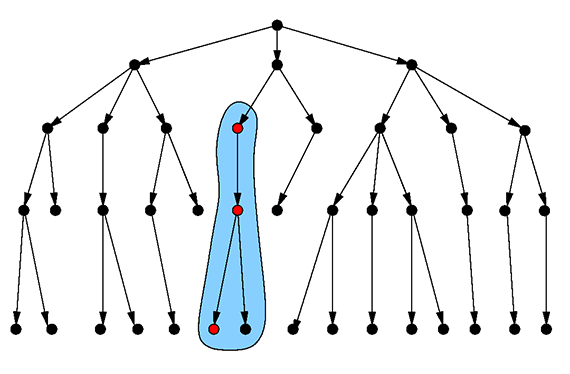
Figure 4: Finding the smallest maintainable component. Image courtesy of Max Neunhöffer.
For example, the following is an AQL query that finds the shortest path from “parts/Screw56744” to a vertex whose isMaintainable attribute has the boolean value true, following the edges in the “inbound” direction:
RETURN GRAPH_SHORTEST_PATH("FleetGraph",
                           "parts/Screw56744",
                           {isMaintainable: true},
                           {direction: "inbound",
                            stopAtFirstMatch: true})
Note that here, we specify the graph name, the _id of the start vertex and a pattern for the target vertex. We could have given a concrete _id instead, or could have given further options in addition to the direction of travel in the last argument. We see again that AQL directly supports this type of graphy query.
- Which parts of this aircraft need maintenance next week?
This is a query that does not involve the graph structure at all: rather, the result tends to be nearly orthogonal to the graph structure. Nevertheless, the document data model with the right secondary index is a perfect fit for this query.
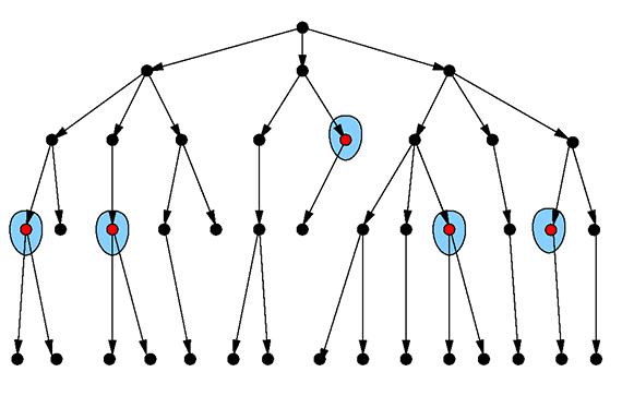
Figure 5: Query whose result is orthogonal to the graph structure. Image courtesy of Max Neunhöffer.
With a pure graph database, we would be in trouble rather quickly for such a query. That is because we cannot use the graph structure in any sensible way, so we have to rely on secondary indexes — here, for example, on the attribute storing the date of the next maintenance. Obviously, a graph database could implement secondary indexes on its vertex data, but then it would essentially become a multi-model database.
To get our answer, we turn to a document query, which does not consider the graph structure. Here is one that finds the components that are due for maintenance:
FOR c IN components
  FILTER c.nextMaintenance <= "2015-05-15"
  RETURN {id: c._id,
          nextMaintenance: c.nextMaintenance}
What looks like a loop is AQL’s way to describe an iteration over the components collection. The query optimiser recognises the presence of a secondary index for the nextMaintenance attribute such that the execution engine does not have to perform a full collection scan to satisfy the FILTER condition. Note AQL’s way to specify projections by simply forming a new JSON document in the RETURN statement from known data. We see that the very same language supports queries usually found in a document store.
Using multi-model querying
To illustrate the potential of the multi-model approach, I’ll finally present an AQL query that mixes the three data models. The following query starts by finding parts with maintenance due, runs the above shortest path computation for each of them, and then performs a join operation with the contacts collection to add concrete contact information to the result:
FOR p IN parts
  FILTER p.nextMaintenance <= "2015-05-15"
  LET path = GRAPH_SHORTEST_PATH("FleetGraph", p._id,
                        {isMaintainable: true},
                        {direction: "inbound",
                         stopAtFirstMatch: true})
  LET pathverts = path[0].vertices
  LET c = DOCUMENT(pathverts[LENGTH(pathverts)-1])
  FOR person IN contacts
    FILTER person._key == c.contact
    RETURN {part: p._id, component: c, contact: person}
In AQL, the DOCUMENT function call performs a key/value lookup via the provided _id attribute; this is done for each vertex found as target of the shortest path computation. Finally, we can see AQL’s formulation for a join. The second FOR statement brings the contacts collection into play, and the query optimiser recognises that the FILTER statement can be satisfied best by doing a join, which in turn is very efficient because it can use the primary index of the contacts collection for a fast hash lookup.
This is a prime example for the potential of the multi-model approach. The query needs all three data models: documents with secondary indexes, graphy queries, and a join powered by fast key/value lookup. Imagine the hoops through which we would have to jump if the three data models would not reside in the same database engine, or if it would not be possible to mix them in the same query.
Even more importantly, this case study shows that the three different data models were indeed necessary to achieve good performance for all queries arising from the application. Without a graph database, the queries of a graphy nature with path lengths, which are not a priori known, notoriously lead to nasty, inefficient multiple join operations. However, a pure graph database cannot satisfy our needs for the document queries that we got efficiently by using the right secondary indexes. The efficient key/value lookups complement the picture by allowing interesting join operations that give us further flexibility in the data modeling. For example, in the above situation, we did not have to embed the whole contact information with every single path, simply because we could perform the join operation in the last query.
Lessons learned for data modeling
The case study of aircraft fleet maintenance reveals several important points about data modeling and multi-model databases.
- JSON is very versatile for unstructured and structured data. The recursive nature of JSON allows embedding of subdocuments and variable length lists. Additionally, you can even store the rows of a table as JSON documents, and modern data stores are so good at compressing data that there is essentially no memory overhead in comparison to relational databases. For structured data, schema validation can be implemented as needed using an extensible HTTP API.
- Graphs are a good data model for relations. In many real world cases, a graph is a very natural data model. It captures relations and can hold label information with each edge and with each vertex. JSON documents are a natural fit to store this type of vertex and edge data.
- A graph database is particularly good for graphy queries. The crucial thing here is that the query language must implement routines like “shortest path” and “graph traversal”, the fundamental capability for these is to access the list of all outgoing or incoming edges of a vertex rapidly.
- A multi-model database can compete with specialised solutions. The particular choice of the three data models: documents, key/value and graph, allows us to combine them in a coherent engine. This combination is no compromise, it can – as a document store – be as efficient as a specialised solution, and it can – as a graph database – be as efficient as a specialised solution (see this blog post for some benchmarks).
- A multi-model database allows you to choose different data models with less operational overhead. Having multiple data models available in a single database engine alleviates some of the challenges of using different data models at the same time, because it means less operational overhead and less data synchronisation, and therefore allows for a huge leap in data modeling flexibility. You suddenly have the option to keep related data together in the same data store, even if it needs different data models. Being able to mix the different data models within a single query increases the options for application design and performance optimizations. And if you choose to split the persistence layer into several different database instances (even if they use the same data model), you still have the benefit of only having to deploy a single technology. Furthermore, a data model lock-in is prevented.
- Multi-model has a larger solution space than relational. Considering all these possibilities for queries, the additional flexibility in data modeling and the benefits of polyglot persistence without the usually ensuing friction, the multi-model approach covers a solution space that is even larger than that of the relational model. This is all-the-more astonishing, since the relational model has dominated the database market as well as the database research for decades.
- Workflow management software often models the dependencies between tasks with a graph, some queries need these dependencies, others ignore them and only look at the remaining data.
- Knowledge graphs are enormous data collections, most queries from expert systems use only the edges and graphy queries, but often enough you needs “orthogonal” queries only considering the vertex data.
- E-commerce systems need to store customer and product data (JSON), shopping carts (key/value), orders and sales (JSON or graph) and data for recommendations (graph), and need a multitude of queries featuring all of these data items.
- Enterprise hierarchies come naturally as graph data and rights management typically needs a mixture of graphy and document queries.
- Social networks are the prime example for large, highly connected graphs and typical queries are graphy, nevertheless, actual applications need additionally queries which totally ignore the social relationship and thus need secondary indexes and possibly joins with key lookups.
- Version management applications usually work with a directed acyclic graph, but also need graphy queries and others.
- Any application that deals with complex, user-defined data structures benefits dramatically from the flexibility of a document store and has often good applications for graph data as well.
Further use cases for multi-model databases
Here are a few more use cases for which multi-model is well suited or even outright necessary:
The future of multi-model databases
Currently there are only two products that are multi-model in the sense used above, making use of JSON, key/value, and graphs: ArangoDB and OrientDB. A few others are marketed under the term “multi-model” (for a complete overview, see the ranking at DB-engines), which support multiple data models, but none of them has graphs and targets the operational domain.
Other players, like MongoDB or Datastax, who have traditionally concentrated on a single data model, show signs of broadening their scope. MongoDB, which is a pure document store, made their storage engine pluggable with the 3.0 release in March 2015. Datastax, a company that produces a commercial product based on the column-based store Apache Cassandra, has recently acquired Aurelius, the company behind the distributed graph database TitanDB. Apple just acquired FoundationDB, a distributed key/value store with multiple “personalities” for different data models layered on top.
The arrival of the new players, as well as the moves of the more established ones, constitute a rather recent trend toward support for multiple data models. At the same time, more and more NoSQL solutions are appearing that rediscover the traditional virtues of relational databases, such as ACID transactions, joins, and relatively strong consistency guarantees.
These are golden times for data modelers and software architects. Stay tuned, watch the exciting new developments in the database market and enjoy the benefits of an unprecedented amount of choice.